This tutorial is to illustrate the functionality of BoulderALE. We have been using BoulderALE to evaluate alignments which are backed by an x-ray crystal structures, therefore we wanted to incorporate a method for scoring alignments based on how well the alignment corresponds to the PDB structure (Reference Sequence), using isostericty. We also wanted a way to collapse the alignment horizontally, to focus primarily on regions of interest, when editing the alignments. When evaluating alignments it is also convenient to visualize the 2D structure and base composition, therefore those features were also implemented in the editor.
This tutorial shows an overview analysis using a tRNA alignment, where the PDB sequence and basepair list was taken from the FR3D website and the feature list was manually generated based on visual inspection of the 3D x-ray crystal structure of PDB:1N77. However, the Pseudoknot tutorial illustrates the appending of a FR3D basepair list and manual generation of a feature list.
To begin this tutorial, you should first download and unzip the tutorial files here. Next, you should proceed to the BoulderALE website (http://microbio.me/boulderale).
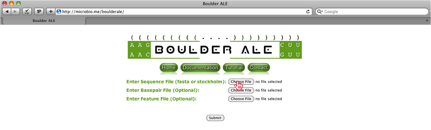
First, you must upload ‘Glu_1N77_Demo.sto’ file to the BoulderALE website, by selecting the “Choose File” input button next to ‘Enter Sequence File’. This file already contains the basepair list extracted from the FR3D website and the manually curated feature list.
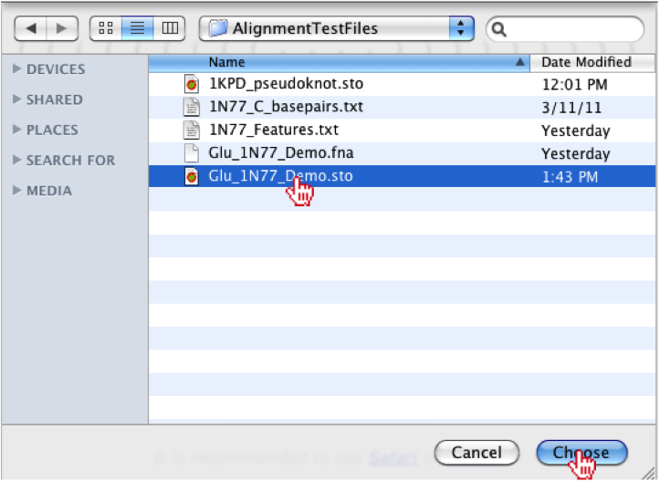
Once the button has been clicked a file menu will appear, where you should select the ‘Glu_1N77_Demo.sto’ file. Once the file is associated, you should click the “Choose” button on the bottom right of the menu.
Note
If the user decides to input the basepair or feature lists, those files, will overwrite the lists present in the STOCKHOLM file.
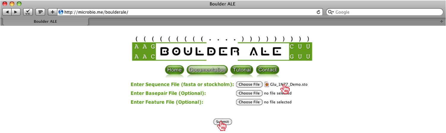
Once the file is chosen, you will see the filename to the right of the “Choose File” button. After selecting file, you should click on the “Submit” button.
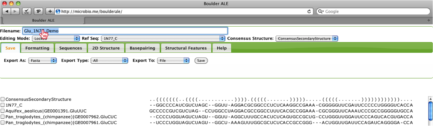
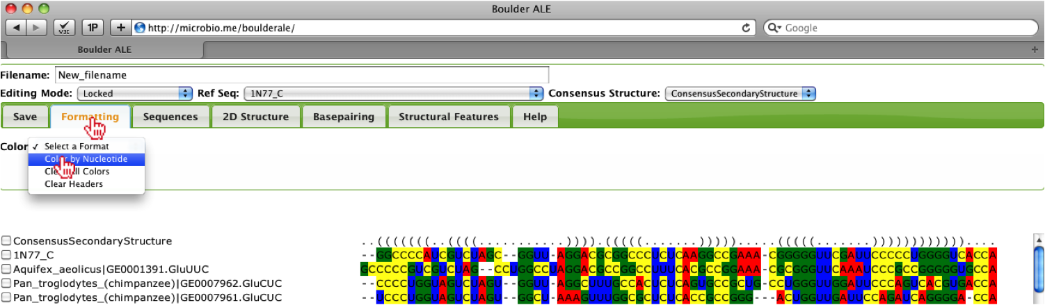
After loading the files, you will be redirected to the alignment. First, you should type in a new filename for the alignment (e.g. New_filename).
To get a brief overview of the base composition in the alignment, you should select the Formatting Tab, followed by Color->Color By Nucleotide. This will color the alignment based on the nucleotide, A (red), C (yellow), G (green) and U (yellow). To remove the colors you can select Color->Clear All Colors.
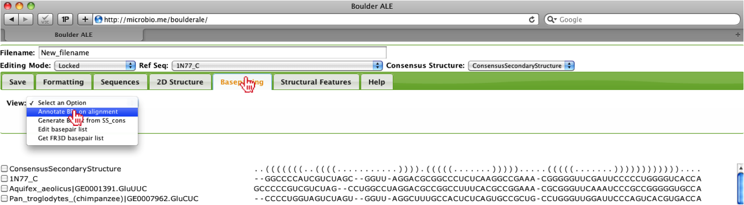
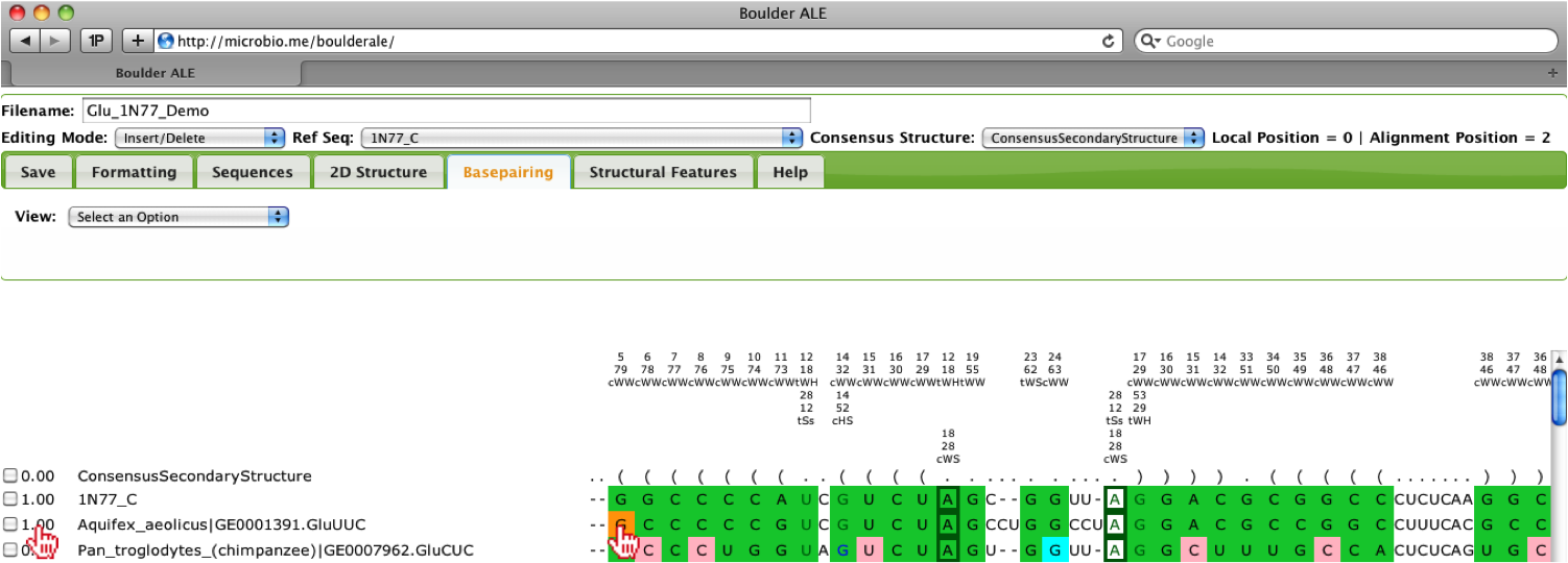
To evaluate the alignment using the basepairs assigned by FR3D to the PDB file: 1N77, you should go to the Basepairing Tab. Evaluation of basepairing (both 2D and 3D) relies on setting a Reference Sequence, if it is not pre-defined in the basepair list. The reason for this is due to our calculations, where we evaluate whether one basepair is isosteric to the Reference Sequence basepair using the IsoDiscrepancy Index defined by [3]. In this example, the basepair list was already in the STOCKHOLM file, however; if the user does not have a basepair list, they can either generate a basepair list using their selected consensus secondary structure (Generate BP list from SS_cons option) or they can get a FR3D basepair list (Get FR3D basepair list option), if there is a corresponding crystal structure to the user’s alignment. User’s will only need to define the Reference Sequence if they generate a new basepair list using the consensus secondary structure or if they supply their own basepair list. The user also has the option of editing their basepair list or manually creating a basepair list (Edit basepair list option).
The alignment will be annotated with the basepairs and you should notice that some bases are involved in more than one basepair, therefore there are multiple rows used for annotating the alignment. The coloring for isosteric [3] (green), non-isosteric (pink), not-allowed (cyan) to the Reference Sequence is still applied, however; you will notice that the cells around the nucleotides are colored slightly differently. Since bases are participating in more than one interactions, we need to show the isostericity of each basepair, so when a basepair is listed in the first 3 rows above the alignment, then the background of the cell is colored. If the basepair is listed in rows 4-6, then the nucleotide text is colored and if listed in rows 7-9, the border is colored. Note: To avoid blending of colors, slight variations of the isostericity colors are applied, such that different shades of green are used for isosteric basepairs. To evaluate how well a sequence corresponds to the reference, you should look at the percent isostericity score for a given sequence, which located between the checkbox and sequence name on the left of the alignment. This calculation is as follows:
percent isosteric = (# of isosteric basepairs)/(Total # of basepairs)
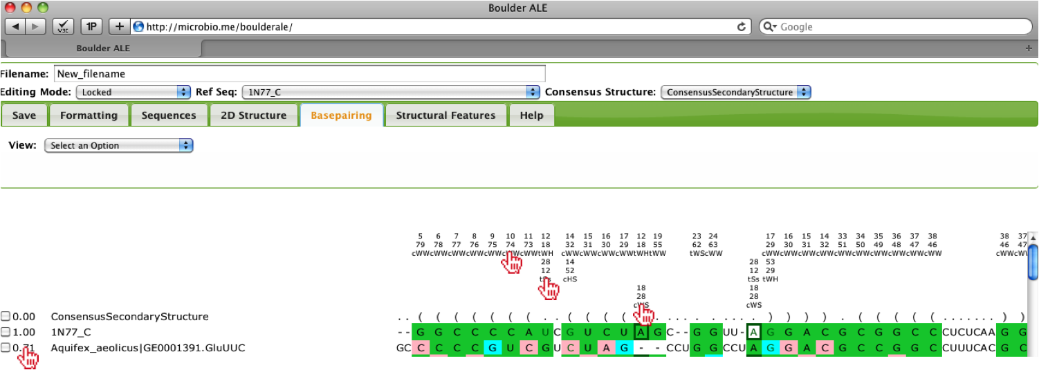
When looking over the alignment you should notice that the third sequence “Aquifex_aeolicus” has a low score (0.71) and it appears that it is slightly misaligned, so to edit the alignment, you should select the Editing Mode “Insert/Delete”. Then, you should select the far left “G” in that sequence.
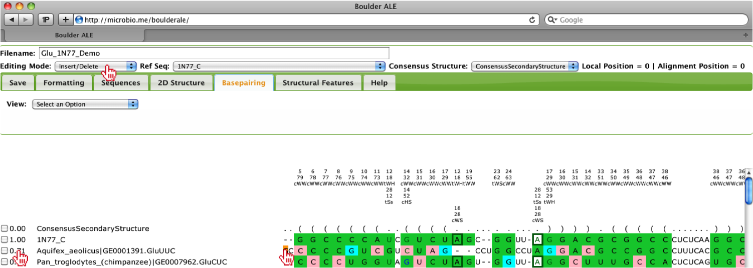
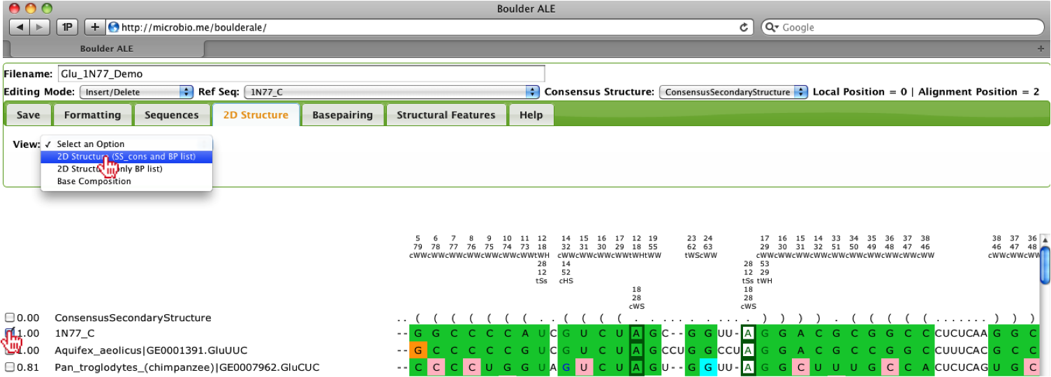
By holding down the Shift key and pressing the Right arrow key, you can slide the “G” to the right two spaces. You should notice that the percent isostericity score increases to 1.00 and you will also notice the colors on the alignment automatically update. You could have also done this procedure by pressing the SpaceBar twice while the “G” was selected.
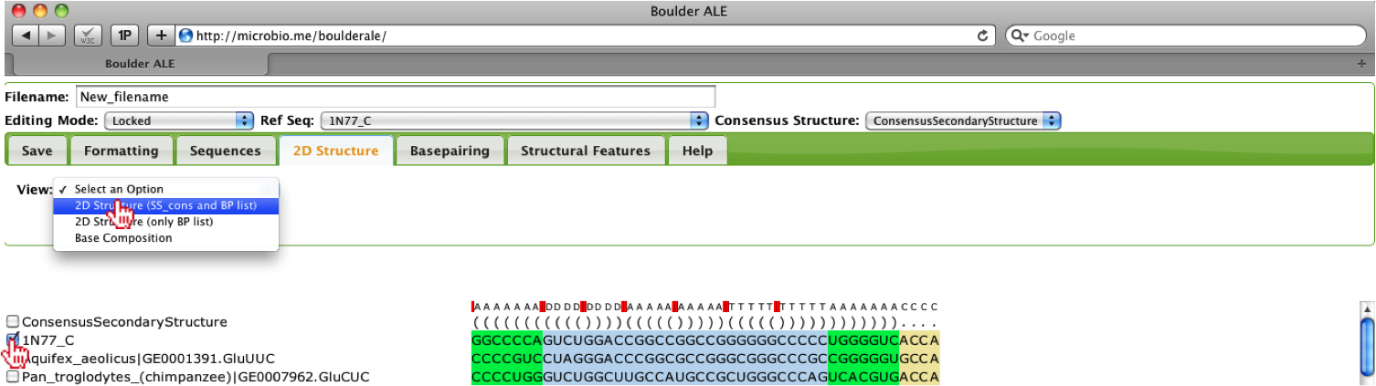
In the case that you want to see how well a particular sequence looks in 2D space, you can view the 2D structure by selecting one of the sequences (checkbox to the left of sequence name) and select View->2D Structure (SS_cons and BP list) under the 2D Structure Tab. The use of the SS_cons takes into account the consensus secondary structure when laying out the image. This feature only works if consensus secondary structure does not contain pseudoknots, otherwise, you should use the 2D Structure (only BP list) option.
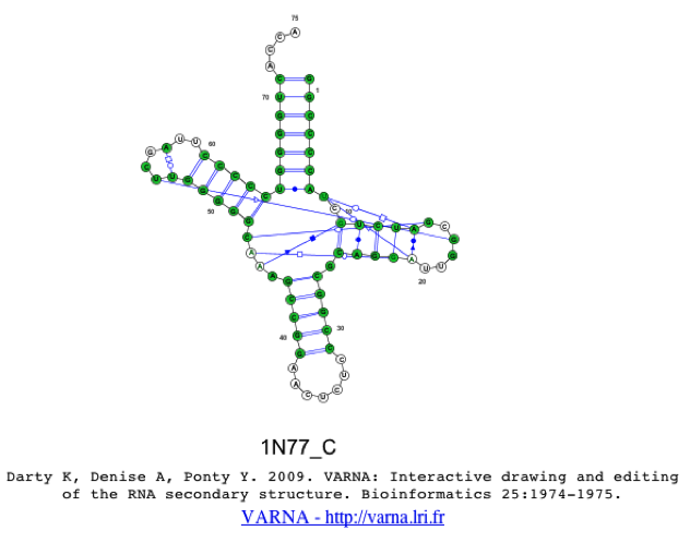
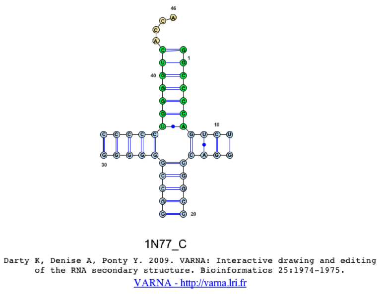
This will produce a 2D structure image using the VARNA java-applet [1], where you can move around the stems, by clicking and dragging. As you will see, when selecting only a single sequence, the colors from the alignment will be transferred to the 2D structure. In the case that the user selects multiple sequences, the colors cannot be transferred due to limitations of opening multiple 2D structures within a single applet. One should also notice that both Watson-Crick and non-Watson-Crick basepairs are represented in the 2D structure, which are based on the Leontis-Westhof annotation schema [4].
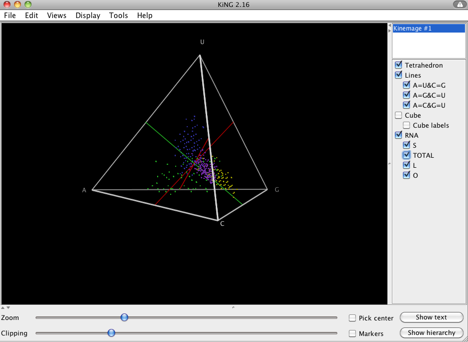
To get a better understanding of nucleotide composition within the stems and loops of the RNA based on your alignment [2], you can select View->Base Composition under the 2D Structure Tab.
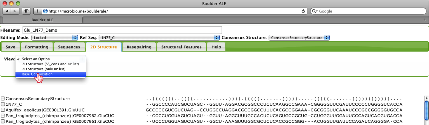
This produces a kinemage file, which is viewable in the KiNG java-applet. In the menu you should see “S”, “L”, “O” and “Total” under the RNA menu, where the letters stand for Stem, Loop, Other, and Total, respectively. You should notice that the stems (yellow) are composed of more G/C’s and the loops (blue) are composed of more U’s.
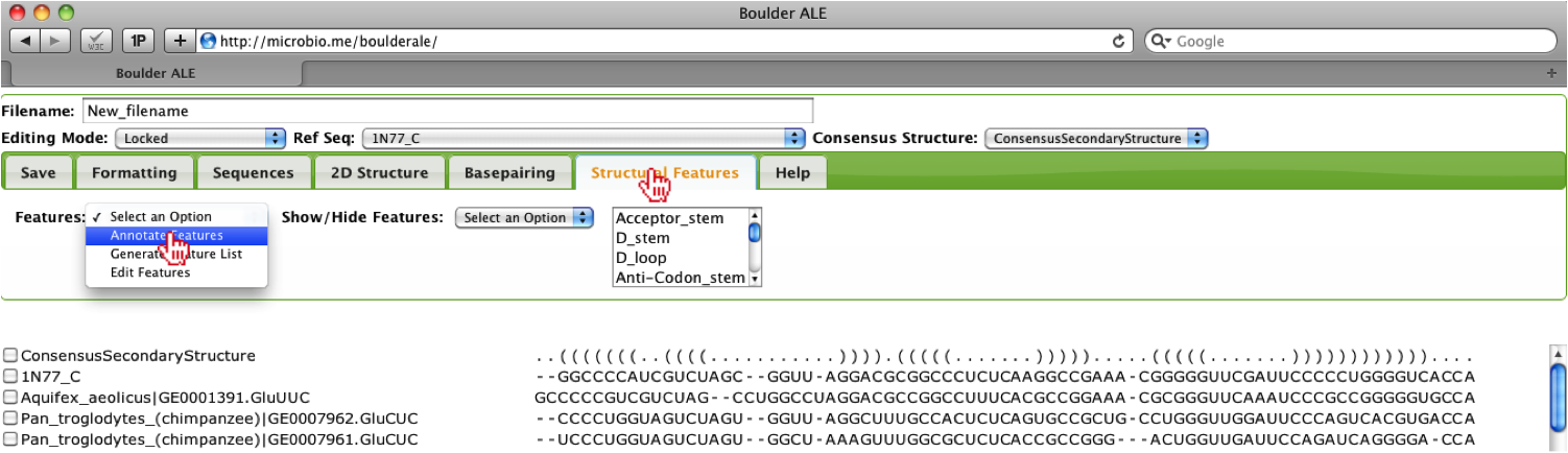
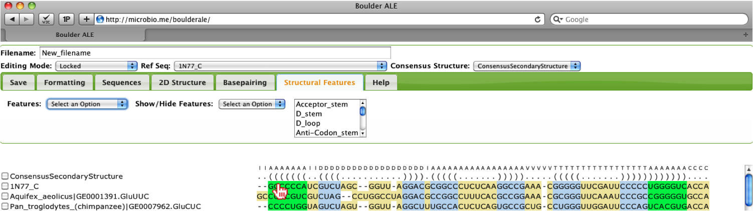
To annotate the alignment with structural features, you should select the “Annotate Features” button under the Structural Features Tab.
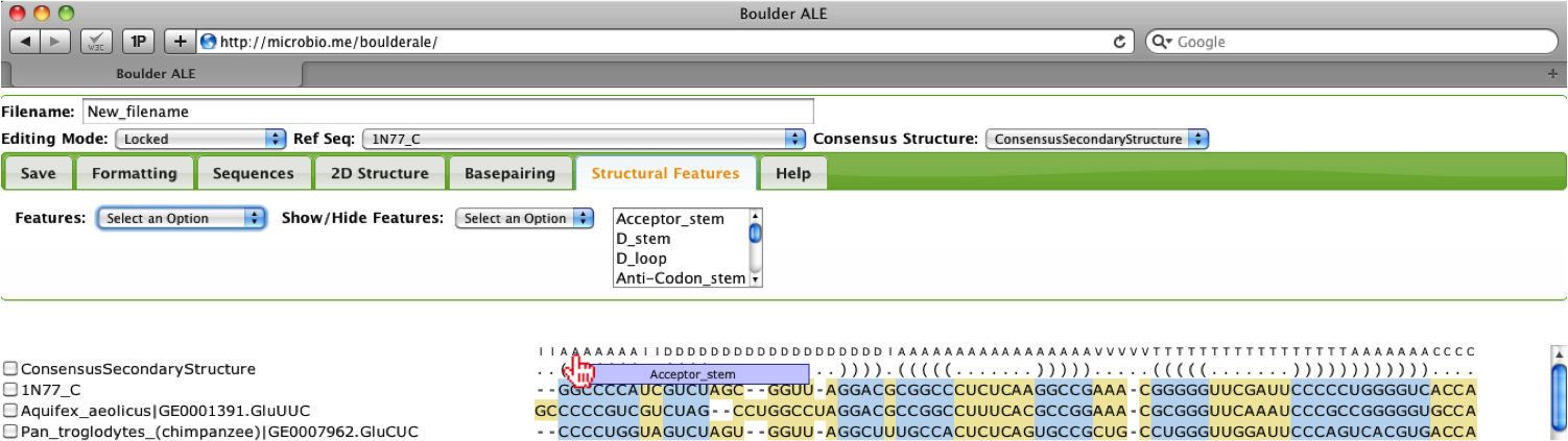
You may need to collapse the Tabs to view the annotations by clicking on the Structural Features Tab. When you mouse over the annotations, you will see the full annotation for that column in the alignment.
Users have the ability to edit the features and to change the color of different features by selecting the Edit features option.
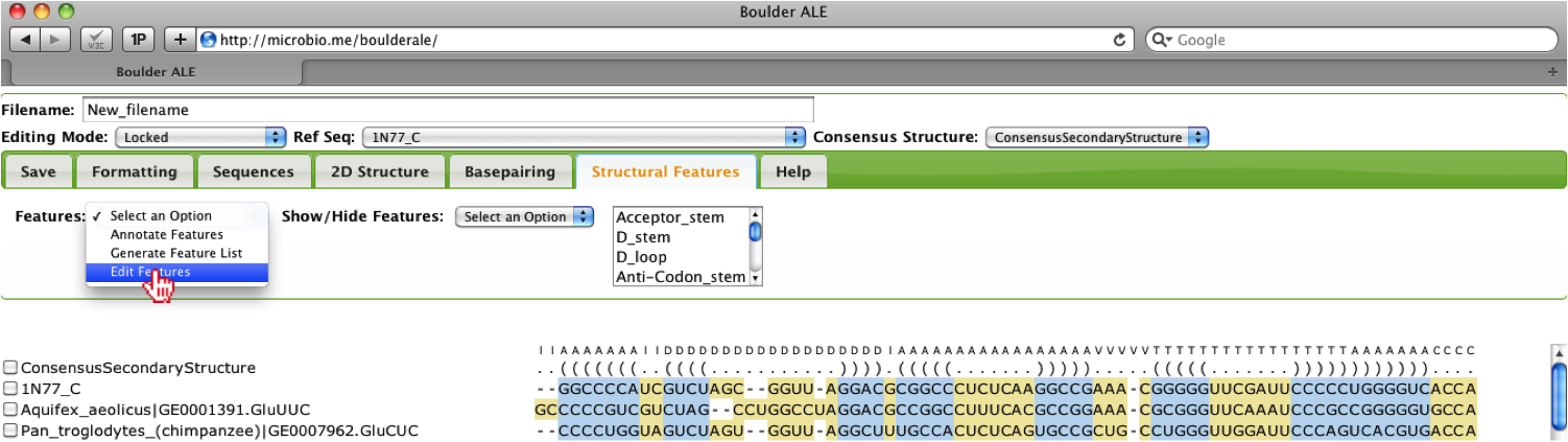
A new console window will appear, where the user will observe the different features assigned to their alignment. Note: the Alignment Range refers to global positions in the alignment. In this window, the user, can add/remove features, change the color of features and edit the names and ranges assigned to each feature. Note: you should not use any spaces in the "Feature Type" and "Feature Name" fields, otherwise the features can not be saved and reloaded. For instance, we can change the color of the Acceptor stem, by clicking on the input box, then select the color of choice. If the user wants all stems to be the same color, they can click on the “C” button, but for this example, we will just change the color of the Acceptor stem and save the features.
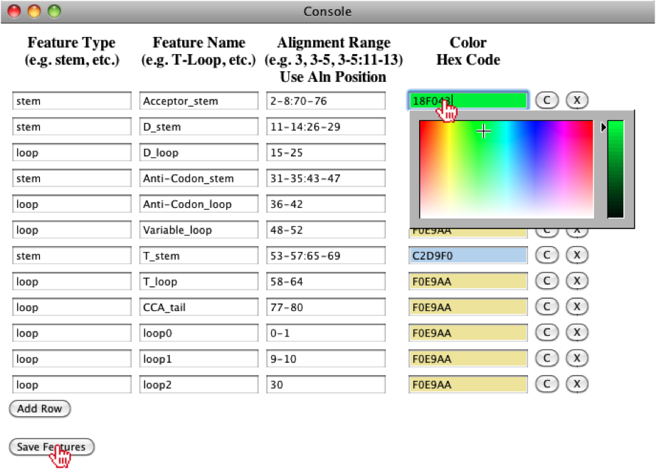
The user should notice that the Acceptor stem in the alignment is now the color selected.
You can collapse features (horizontally) by selecting the features from the multi-select box (e.g. all features with the word “loop” in their name) and then selecting Hide option.
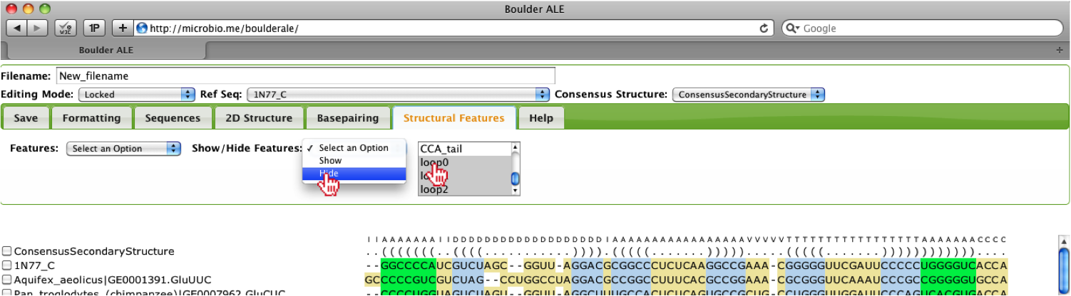
You should notice that all the features selected have been collapsed and are no longer visible (red lines above the alignment denote locations of collapsed features. You can edit the alignment in this mode and to make the feature visible they should make sure the features are selected, then select the Show option.
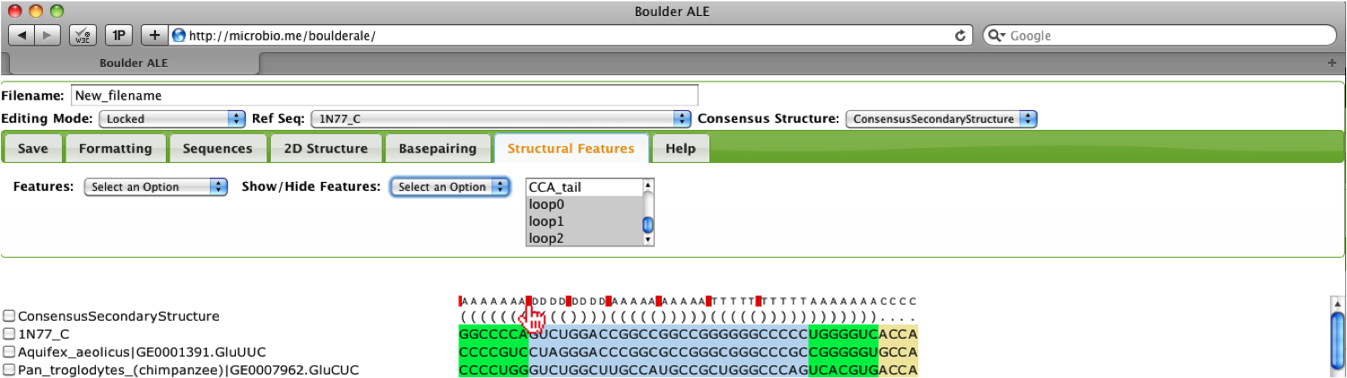
Users also have the option of re-annotating the basepairs onto the collapsed alignment, so they can evaluate the isostericity of the visible regions.
Alternatively, users can visualize the 2D structure for the visible regions of the alignment. This can be very useful if there are specific alignment regions full of gaps or for focusing on a particular motif. While the alignment is collapsed, the user can select a sequence(s), then select 2D Structure (SS_cons and BP list) from the 2D Structure Tab.
This will produce a 2D structure containing only the visible parts of the alignment.
To save an alignment, users should go to the Save Tab, where they are given 3 options: 1) Export As (FASTA or STOCKHOLM); 2) Export Type (whether to export all sequence data, or just the visible sequence data); and 3) Export To (new window or file). Once the user has selected their options they should click on the Save button.

| [1] | Darty K, Denise A, Ponty Y. 2009. VARNA: Interactive drawing and editing of the RNA secondary structure. Bioinformatics 25:1974-1975. |
| [2] | Smit S, Knight R, Heringa J. 2009. RNA structure prediction from evolutionary patterns of nucleotide composition. Nucleic acids research 37:1378-1386. |
| [3] | (1, 2) Stombaugh, J., Zirbel, C. L., Westhof, E., & Leontis, N. B. (2009). Frequency and isostericity of RNA base pairs. Nucleic Acids Res, 37(7), 2294-2312. |
| [4] | Leontis, N. B., & Westhof, E. (2001). Geometric nomenclature and classification of RNA base pairs. RNA, 7(4), 499-512. |